EDA 프로젝트
Mission : It’s Your Turn!
1. 본문에서 언급된 Feature를 제외하고 유의미한 Feature를 1개 이상 찾아봅시다.
- Hint : Fare? Sibsp? Parch?
2. Kaggle에서 Dataset을 찾고, 이 Dataset에서 유의미한 Feature를 3개 이상 찾고 이를 시각화해봅시다.
함께 보면 좋은 라이브러리 document
무대뽀로 하기 힘들다면? 다음 Hint와 함께 시도해봅시다:
- 데이터를 톺아봅시다.
- 각 데이터는 어떤 자료형을 가지고 있나요?
- 데이터에 결측치는 없나요? -> 있다면 이를 어떻게 메꿔줄까요?
- 데이터의 자료형을 바꿔줄 필요가 있나요? -> 범주형의 One-hot encoding
- 데이터에 대한 가설을 세워봅시다.
- 가설은 개인의 경험에 의해서 도출되어도 상관이 없습니다.
- 가설은 명확할 수록 좋습니다. ex) Titanic Data에서 Survival 여부와 성별에는 상관관계가 있다!
- 가설을 검증하기 위한 증거를 찾아봅시다.
- 이 증거는 한 눈에 보이지 않을 수 있습니다. 우리가 다룬 여러 Technique를 써줘야 합니다.
groupby()를 통해서 그룹화된 정보에 통계량을 도입하면 어떨까요?- 시각화를 통해 일목요연하게 보여주면 더욱 좋겠죠?
# 라이브러리 선언
import pandas as pd
import numpy as np
import matplotlib.pyplot as plt
import seaborn as sns

%matplotlib inline
# 데이터 불러오기
data = pd.read_csv('./bestsellers with categories.csv')
data.head()
| Name | Author | User Rating | Reviews | Price | Year | Genre | |
|---|---|---|---|---|---|---|---|
| 0 | 10-Day Green Smoothie Cleanse | JJ Smith | 4.7 | 17350 | 8 | 2016 | Non Fiction |
| 1 | 11/22/63: A Novel | Stephen King | 4.6 | 2052 | 22 | 2011 | Fiction |
| 2 | 12 Rules for Life: An Antidote to Chaos | Jordan B. Peterson | 4.7 | 18979 | 15 | 2018 | Non Fiction |
| 3 | 1984 (Signet Classics) | George Orwell | 4.7 | 21424 | 6 | 2017 | Fiction |
| 4 | 5,000 Awesome Facts (About Everything!) (Natio... | National Geographic Kids | 4.8 | 7665 | 12 | 2019 | Non Fiction |
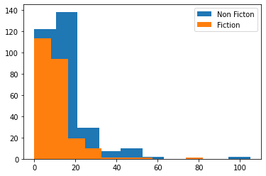
# Non Fiction과 Fiction장르의 가격차이

plt.hist(data[data['Genre']=='Non Fiction']['Price'])
plt.hist(data[data['Genre']=='Fiction']['Price'])
plt.legend(['Non Ficton', 'Fiction'])

plt.show()
# 전반적으로 Non Fiction인 책이 Fiction인 책보다 가격대가 높음을 알 수 있다.
# Non Fiction인 책의 경우 전문서적 등이 많이 포함되어 Fiction인 책보다 가격대가 높은 게 않을까?
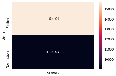
# Non Fiction과 Fiction장르의 리뷰차이
sns.heatmap(data[['Genre','Reviews']].groupby(['Genre']).mean(), annot=True)
plt.show()
# Fiction이 Non Fiction보다 리뷰가 많은 것을 알 수 있다.
sns.heatmap(data.corr(), annot=True)
plt.show()
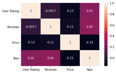
음.. 딱히 건져낼만한 유의미한 Feature을 더 찾기 힘들어서 다른 데이터셋으로 해보았다. 강한 상관관계가 보이지 않는다.
상관계수에 대하여
- -1에 가까운 값이 얻어지면 : 누가 봐도 매우 강력한 음(-)의 상관. 오히려 너무 확고하기 때문에 사회과학 데이터일 경우 데이터를 조작한 게 아닌가 의심할 정도이다. 물론 이건 사회과학 얘기고 순수학문에 가까운 분야일수록 요구되는 상관관계는 높은 편.
- -0.5 정도의 값이 얻어지면 : 강력한 음(-)의 상관. 연구자는 변인 x 가 증가하면 변인 y 가 감소한다고 자신 있게 말할 수 있다.
- -0.2 정도의 값이 얻어지면 : 음(-)의 상관이긴 한데 너무 약해서 모호하다. 상관관계가 없다고는 할 수 없지만 좀 더 의심해 봐야 한다.
- 0 정도의 값이 얻어지면 : 대부분의 경우, 상관관계가 있을거라고 간주되지 않는다. 다른 후속 연구들을 통해 뒤집어질지는 모르지만 일단은 회의적이다. 하지만 무조건적으로 그런건 아니라 2차 방정식 그래프와 비슷한 모양이 될 경우 상관관계는 있으나 상관계수는 0에 가깝게 나온다.
- 0.2 정도의 값이 얻어지면 : 너무 약해서 의심스러운 양(+)의 상관. 이것만으로는 상관관계에 대해 아주 장담할 수는 없다. 하지만 사회과학에선 매우 큰 상관관계가 있는 것으로 간주한다.
- 0.5 정도의 값이 얻어지면 : 강력한 양(+)의 상관. 변인 x 가 증가하면 변인 y 가 증가한다는 주장은 이제 통계적으로 지지받고 있다.
- 1에 가까운 값이 얻어지면 : 이상할 정도로 강력한 양(+)의 상관. 위와 마찬가지로, 이렇게까지 확고한 상관관계는 오히려 쉽게 찾아보기 어렵다.
Word Happiness Report 데이터셋
https://pandas.pydata.org/docs/reference/api/pandas.DataFrame.drop.html
- pandas API레퍼런스
http://seaborn.pydata.org/generated/seaborn.displot.html#seaborn.displot
- seaborn API레퍼런스
data15 = pd.read_csv('./word_happiness_report/2015.csv')
data16 = pd.read_csv('./word_happiness_report/2016.csv')
data17 = pd.read_csv('./word_happiness_report/2017.csv')
data18 = pd.read_csv('./word_happiness_report/2018.csv')
data19 = pd.read_csv('./word_happiness_report/2019.csv')
# data = pd.concat([data15,data16,data17,data18,data19])
# data
# sns.heatmap(data.corr(), annot=True)
# 위와 같이 5개의 데이터를 한번에 합쳤더니 column도 다 다르고, 결측치도 많아서 엄청나게 더러워졌다 ㅠ
# 일단 각 column을 살펴보면서 정리해줘야겠다! 버릴 건 drop하고, 의미가 같지만 이름이 다른 column끼리는 통합해주고.
data15.head(5)
# Standard Error는 2015년에만 존재한다.
# Dystopia Residual도 2015년과 2016년에만 존재한다. 2017년의 Dystopia.Residual와 같다.
# Region은 2015, 2016년에만 있다.
# Country는 다른 연도의 Country or region과 같은 내용을 담고 있다.
# Overall rank == Happiness Rank
| Country | Region | Happiness Rank | Happiness Score | Standard Error | Economy (GDP per Capita) | Family | Health (Life Expectancy) | Freedom | Trust (Government Corruption) | Generosity | Dystopia Residual | |
|---|---|---|---|---|---|---|---|---|---|---|---|---|
| 0 | Switzerland | Western Europe | 1 | 7.587 | 0.03411 | 1.39651 | 1.34951 | 0.94143 | 0.66557 | 0.41978 | 0.29678 | 2.51738 |
| 1 | Iceland | Western Europe | 2 | 7.561 | 0.04884 | 1.30232 | 1.40223 | 0.94784 | 0.62877 | 0.14145 | 0.43630 | 2.70201 |
| 2 | Denmark | Western Europe | 3 | 7.527 | 0.03328 | 1.32548 | 1.36058 | 0.87464 | 0.64938 | 0.48357 | 0.34139 | 2.49204 |
| 3 | Norway | Western Europe | 4 | 7.522 | 0.03880 | 1.45900 | 1.33095 | 0.88521 | 0.66973 | 0.36503 | 0.34699 | 2.46531 |
| 4 | Canada | North America | 5 | 7.427 | 0.03553 | 1.32629 | 1.32261 | 0.90563 | 0.63297 | 0.32957 | 0.45811 | 2.45176 |
data16.head(5)
# Dystopia Residual도 2015년과 2016년에만 존재한다. 2017년의 Dystopia.Residual와 같다.
# Region은 2015, 2016년에만 있다.
# Country는 다른 연도의 Country or region과 같은 내용을 담고 있다.
# Lower Confidence Interval은 2016년에만 있다.
# Upper Confidence Interval도 2016년에만 있다.
# Overall rank == Happiness Rank
| Country | Region | Happiness Rank | Happiness Score | Lower Confidence Interval | Upper Confidence Interval | Economy (GDP per Capita) | Family | Health (Life Expectancy) | Freedom | Trust (Government Corruption) | Generosity | Dystopia Residual | |
|---|---|---|---|---|---|---|---|---|---|---|---|---|---|
| 0 | Denmark | Western Europe | 1 | 7.526 | 7.460 | 7.592 | 1.44178 | 1.16374 | 0.79504 | 0.57941 | 0.44453 | 0.36171 | 2.73939 |
| 1 | Switzerland | Western Europe | 2 | 7.509 | 7.428 | 7.590 | 1.52733 | 1.14524 | 0.86303 | 0.58557 | 0.41203 | 0.28083 | 2.69463 |
| 2 | Iceland | Western Europe | 3 | 7.501 | 7.333 | 7.669 | 1.42666 | 1.18326 | 0.86733 | 0.56624 | 0.14975 | 0.47678 | 2.83137 |
| 3 | Norway | Western Europe | 4 | 7.498 | 7.421 | 7.575 | 1.57744 | 1.12690 | 0.79579 | 0.59609 | 0.35776 | 0.37895 | 2.66465 |
| 4 | Finland | Western Europe | 5 | 7.413 | 7.351 | 7.475 | 1.40598 | 1.13464 | 0.81091 | 0.57104 | 0.41004 | 0.25492 | 2.82596 |
data17.head(5)
# Country는 다른 연도의 Country or region과 같은 내용을 담고 있다.
# Whisker.high는 2017년에만 있다.
# Whisker.low도 2017년에만 있다.
# Dystopia.Residual는 2017년에만 있다. 2015,1016년의 Dystopia Residual와 같다.
# Overall rank == Happiness Rank
| Country | Happiness.Rank | Happiness.Score | Whisker.high | Whisker.low | Economy..GDP.per.Capita. | Family | Health..Life.Expectancy. | Freedom | Generosity | Trust..Government.Corruption. | Dystopia.Residual | |
|---|---|---|---|---|---|---|---|---|---|---|---|---|
| 0 | Norway | 1 | 7.537 | 7.594445 | 7.479556 | 1.616463 | 1.533524 | 0.796667 | 0.635423 | 0.362012 | 0.315964 | 2.277027 |
| 1 | Denmark | 2 | 7.522 | 7.581728 | 7.462272 | 1.482383 | 1.551122 | 0.792566 | 0.626007 | 0.355280 | 0.400770 | 2.313707 |
| 2 | Iceland | 3 | 7.504 | 7.622030 | 7.385970 | 1.480633 | 1.610574 | 0.833552 | 0.627163 | 0.475540 | 0.153527 | 2.322715 |
| 3 | Switzerland | 4 | 7.494 | 7.561772 | 7.426227 | 1.564980 | 1.516912 | 0.858131 | 0.620071 | 0.290549 | 0.367007 | 2.276716 |
| 4 | Finland | 5 | 7.469 | 7.527542 | 7.410458 | 1.443572 | 1.540247 | 0.809158 | 0.617951 | 0.245483 | 0.382612 | 2.430182 |
data18.head(5)
# Country or region은 다른 연도의 Country와 같은 내용을 담고 있다.
# Overall rank == Happiness Rank
| Overall rank | Country or region | Score | GDP per capita | Social support | Healthy life expectancy | Freedom to make life choices | Generosity | Perceptions of corruption | |
|---|---|---|---|---|---|---|---|---|---|
| 0 | 1 | Finland | 7.632 | 1.305 | 1.592 | 0.874 | 0.681 | 0.202 | 0.393 |
| 1 | 2 | Norway | 7.594 | 1.456 | 1.582 | 0.861 | 0.686 | 0.286 | 0.340 |
| 2 | 3 | Denmark | 7.555 | 1.351 | 1.590 | 0.868 | 0.683 | 0.284 | 0.408 |
| 3 | 4 | Iceland | 7.495 | 1.343 | 1.644 | 0.914 | 0.677 | 0.353 | 0.138 |
| 4 | 5 | Switzerland | 7.487 | 1.420 | 1.549 | 0.927 | 0.660 | 0.256 | 0.357 |
data19.head(5)
# Country or region은 다른 연도의 Country와 같은 내용을 담고 있다.
# Overall rank == Happiness Rank
| Overall rank | Country or region | Score | GDP per capita | Social support | Healthy life expectancy | Freedom to make life choices | Generosity | Perceptions of corruption | |
|---|---|---|---|---|---|---|---|---|---|
| 0 | 1 | Finland | 7.769 | 1.340 | 1.587 | 0.986 | 0.596 | 0.153 | 0.393 |
| 1 | 2 | Denmark | 7.600 | 1.383 | 1.573 | 0.996 | 0.592 | 0.252 | 0.410 |
| 2 | 3 | Norway | 7.554 | 1.488 | 1.582 | 1.028 | 0.603 | 0.271 | 0.341 |
| 3 | 4 | Iceland | 7.494 | 1.380 | 1.624 | 1.026 | 0.591 | 0.354 | 0.118 |
| 4 | 5 | Netherlands | 7.488 | 1.396 | 1.522 | 0.999 | 0.557 | 0.322 | 0.298 |
이제 모든 연도에 있지 않은 column들은 삭제해줄건데, del과 drop중 뭐를 쓰는게 좋을지 몰라서 찾아봤다.
del은 “remove an item from a list”라며 list를 기준으로 remove가 일어납니다. drop은 pandas.DataFrame.drop method로서 pandas에 특화되어 있기 때문에 drop을 사용하는걸 추천드립니다.
라고 나오길래 drop을 쓰기로 했다..!
사용된 파라미터는 다음과 같다(판다스 API레퍼런스에 의하면..)
- columnssingle label or list-like
- Alternative to specifying axis (labels, axis=1 is equivalent to columns=labels).
- nplacebool, default False
- If False, return a copy. Otherwise, do operation inplace and return None.
- errors{‘ignore’, ‘raise’}, default ‘raise’
- If ‘ignore’, suppress error and only existing labels are dropped.
- axis{0 or ‘index’, 1 or ‘columns’}, default 0
- Whether to drop labels from the index (0 or ‘index’) or columns (1 or ‘columns’).
data15.drop(columns="Standard Error",inplace=True,errors="ignore", axis=1)
data15.drop(columns="Dystopia Residual",inplace=True,errors="ignore", axis=1)
data15.drop(columns="Region",inplace=True,errors="ignore", axis=1)

data16.drop(columns="Lower Confidence Interval",inplace=True,errors="ignore", axis=1)
data16.drop(columns="Upper Confidence Interval",inplace=True,errors="ignore", axis=1)
data16.drop(columns="Dystopia Residual",inplace=True,errors="ignore", axis=1)
data16.drop(columns="Region",inplace=True,errors="ignore", axis=1)

data17.drop(columns="Whisker.high",inplace=True,errors="ignore", axis=1)
data17.drop(columns="Whisker.low",inplace=True,errors="ignore", axis=1)
data17.drop(columns="Dystopia.Residual",inplace=True,errors="ignore", axis=1)
이제 모든 연도에 공통적으로 있는 column들만 남았다. 근데 같은 내용을 담고 있는 column들이라도 이름이 다른 경우가 있어 통일해줘야한다(노가다)
data15=data15.rename(columns={"Country" : "Country or region",
                            "Economy (GDP per Capita)":"GDP per capita",
                            "Health (Life Expectancy)":"Healthy life expectancy",
                            "Trust (Government Corruption)":"Perceptions of corruption"})
data16=data16.rename(columns={"Country" : "Country or region",
                            "Economy (GDP per Capita)":"GDP per capita",
                            "Health (Life Expectancy)":"Healthy life expectancy",
                            "Trust (Government Corruption)":"Perceptions of corruption"})
data17=data17.rename(columns={"Country" : "Country or region",
                            "Happiness.Score":"Happiness Score",
                            "Economy..GDP.per.Capita.":"GDP per capita",
                            "Health..Life.Expectancy.":"Healthy life expectancy",
                            "Trust..Government.Corruption.":"Perceptions of corruption",
                             "Happiness.Rank" : "Happiness Rank"})
data18=data18.rename(columns={"Freedom to make life choices" : "Freedom",
                             "Score" : "Happiness Score",
                             "Social support" : "Family",
                             "Overall rank" : "Happiness Rank"})
data19=data19.rename(columns={"Freedom to make life choices" : "Freedom",
                             "Score" : "Happiness Score",
                             "Social support" : "Family",
                             "Overall rank" : "Happiness Rank"})
alldata = pd.concat([data15,data16,data17,data18,data19])
alldata
| Country or region | Happiness Rank | Happiness Score | GDP per capita | Family | Healthy life expectancy | Freedom | Perceptions of corruption | Generosity | |
|---|---|---|---|---|---|---|---|---|---|
| 0 | Switzerland | 1 | 7.587 | 1.39651 | 1.34951 | 0.94143 | 0.66557 | 0.41978 | 0.29678 |
| 1 | Iceland | 2 | 7.561 | 1.30232 | 1.40223 | 0.94784 | 0.62877 | 0.14145 | 0.43630 |
| 2 | Denmark | 3 | 7.527 | 1.32548 | 1.36058 | 0.87464 | 0.64938 | 0.48357 | 0.34139 |
| 3 | Norway | 4 | 7.522 | 1.45900 | 1.33095 | 0.88521 | 0.66973 | 0.36503 | 0.34699 |
| 4 | Canada | 5 | 7.427 | 1.32629 | 1.32261 | 0.90563 | 0.63297 | 0.32957 | 0.45811 |
| ... | ... | ... | ... | ... | ... | ... | ... | ... | ... |
| 151 | Rwanda | 152 | 3.334 | 0.35900 | 0.71100 | 0.61400 | 0.55500 | 0.41100 | 0.21700 |
| 152 | Tanzania | 153 | 3.231 | 0.47600 | 0.88500 | 0.49900 | 0.41700 | 0.14700 | 0.27600 |
| 153 | Afghanistan | 154 | 3.203 | 0.35000 | 0.51700 | 0.36100 | 0.00000 | 0.02500 | 0.15800 |
| 154 | Central African Republic | 155 | 3.083 | 0.02600 | 0.00000 | 0.10500 | 0.22500 | 0.03500 | 0.23500 |
| 155 | South Sudan | 156 | 2.853 | 0.30600 | 0.57500 | 0.29500 | 0.01000 | 0.09100 | 0.20200 |
782 rows × 9 columns
sns.heatmap(alldata.corr(), annot=True)
<AxesSubplot:>
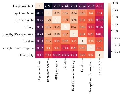
이제 깔끔하게 2015~20019년도를 합쳐서 column간의 상관관계를 파악할 수 있다!!
강한 상관관계를 갖는 column들 중, -0.5 또는 0.5에 가까운 값을 갖는 것들
- Happiness Score & Freedom : 0.55
- GDP per capita & Family : 0.59
- Family & Freedom : 0.42
- Healthy life expectanacy & Family : 0.57
- Freedom & Perception of corruption : 0.46
- Freedom & Happiness Rank : -0.54
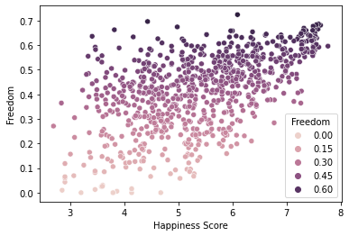
1. Happiness Score & Freedom : 0.55
sns.scatterplot(x='Happiness Score', y='Freedom', hue='Freedom', data=alldata)
plt.xlabel('Happiness Score')
plt.ylabel('Freedom')
plt.show()

# 행복지수가 높을수록 자유롭다고 느끼는 사람이 많음을 알 수 있다.
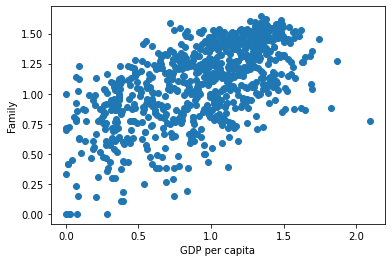
2. GDP per capita & Family : 0.59
plt.scatter(x=alldata['GDP per capita'], y=alldata['Family'])
plt.xlabel('GDP per capita')
plt.ylabel('Family')
plt.show()

# 1인당 GDP 지수가 높을수록 가족이 많은 경우가 많음을 알 수 있다.
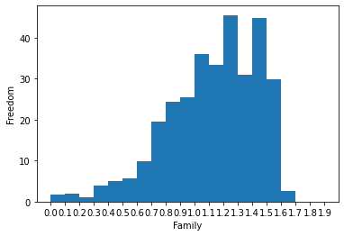
3. Family & Freedom : 0.42
plt.xlabel('Family')
plt.ylabel('Freedom')
plt.hist(x=alldata['Family'], weights=alldata['Freedom'], bins=np.arange(0, 2, 0.1))
plt.xticks(np.arange(0, 2, 0.1)) # Extra : xticks를 올바르게 처리해봅시다.
plt.show()

# 가족이 많을수록 자유를 느끼는 사람들이 많음을 알 수 있다.
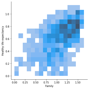
4. Healthy life expectancy & Family : 0.57
sns.displot(data=alldata, x='Family', y='Healthy life expectancy')
plt.show()

# 가족이 많을수록, 건강한 삶에 대한 기대치가 높음을 알 수 있다.
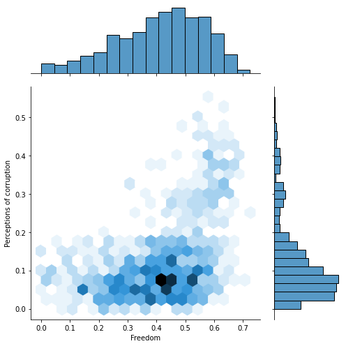
5. Freedom & Perceptions of corruption : 0.46
sns.jointplot(alldata['Freedom'],alldata['Perceptions of corruption'],kind="hex",size=7,ratio=3)
plt.show()

# 자유도가 높다고 해서 반드시 국가가 부패했다는 인식이 높은 것은 아니다.
# 하지만 비교적 자유도가 높을 때, 자유도가 낮을 때보다 국가가 부패했다는 비판적인 인식을 갖고 있는 사람들이 많음을 알 수 있다.
# 그리고 자유도가 높을수록 국가의 부패인식 정도가 0부터 0.5까지 넓게 분포하는 것을 통해,
# 자유도가 높을수록 국가의 부패인식에 대해 다양한 생각을 갖고 있는 사람이 많음을 알 수 있다.
/usr/local/lib/python3.9/site-packages/seaborn/_decorators.py:36: FutureWarning: Pass the following variables as keyword args: x, y. From version 0.12, the only valid positional argument will be `data`, and passing other arguments without an explicit keyword will result in an error or misinterpretation.
  warnings.warn(
/usr/local/lib/python3.9/site-packages/seaborn/axisgrid.py:2015: UserWarning: The `size` parameter has been renamed to `height`; please update your code.
  warnings.warn(msg, UserWarning)
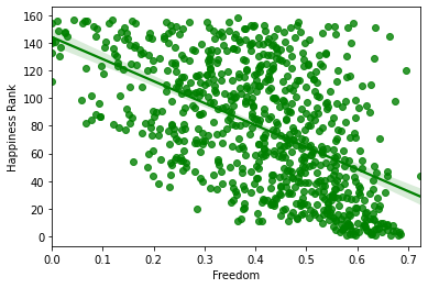
6. Freedom & Happiness Rank : -0.54
sns.regplot(alldata['Freedom'],alldata['Happiness Rank'], color="g")
plt.show()
# 자유도가 높을수록 비교적 행복 순위가 떨어지는 경향을 보임을 알 수 있다.
/usr/local/lib/python3.9/site-packages/seaborn/_decorators.py:36: FutureWarning: Pass the following variables as keyword args: x, y. From version 0.12, the only valid positional argument will be `data`, and passing other arguments without an explicit keyword will result in an error or misinterpretation.
  warnings.warn(